Ball and Beam System
The ball and beam system is a classic benchmark problem in control engineering that is widely used to analyze and evaluate feedback control strategies.
System Description
The system consists of:
- A beam that rotates about a pivot point
- A ball that rolls along the beam under the influence of gravity
- An actuator (such as a motor or servo) that adjusts the beam angle
- A sensor that measures the position of the ball along the beam
By changing the angle of the beam, the position of the ball can be controlled.
Importance in Control Engineering
The ball and beam system is:
- Open loop unstable: without feedback control, the ball will roll off the beam
- Nonlinear: due to trigonometric relationships and rolling dynamics
- Underactuated: the ball position is controlled indirectly through the beam angle
Applications
This system is commonly used for:
- Teaching classical and modern control methods (PID, state space, LQR, nonlinear control)
- Validating control algorithms in simulation and experiments
- Demonstrating concepts such as stability, feedback, and robustness
Simulation Setup in MATLAB and Simulink
To simulate the ball and beam system, the MATLAB and Simulink software environment is used. In the first step, after opening a Blank Model in the Simulink environment of MATLAB, the initial simulation settings must be configured. These include the sampling time, the solver type, and the initialization of the system model parameters.
To set the sampling time and the solver type, right click on the model workspace and select the Model Configuration Parameters option. In the Solver Selection section, set the solver type to Fixed Step and assign the sampling time as Ts. Figure 1 provides a suitable guide for performing these steps.
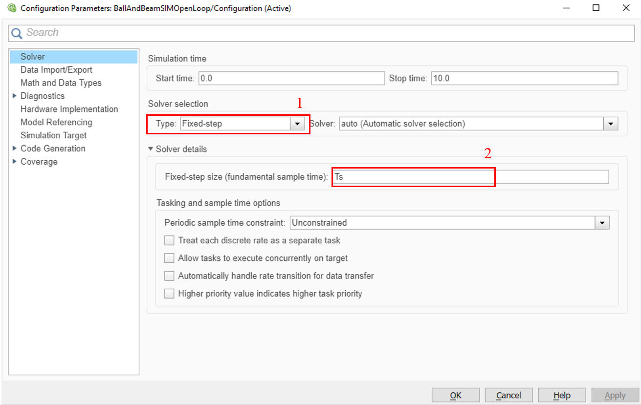
Figure 1. Solver settings and sampling time in the simulation.
Next, it is necessary to enter the initial values of the system model. To do this, right-click on the canvas, open the Model Properties, go to the Callbacks section, and enter the parameters in the InitFcn field as shown in Figure 2.
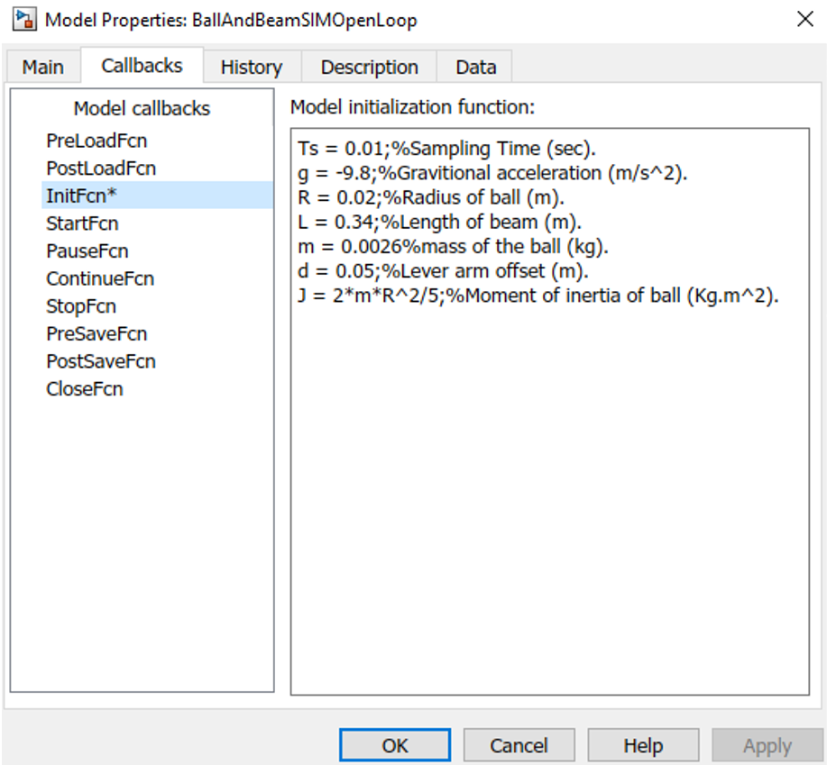
Figure 2. Setting the initial values of the system model.
It is necessary to use the SIMULINK library to add the components required for implementing the model, providing the appropriate input, and displaying the system output. For this purpose, in the Library Browser, under the Continuous, Source, and Sink sections, you can add the transfer function, step input, and output display (Scope) to the simulation environment, respectively. Figure 3 shows this section.
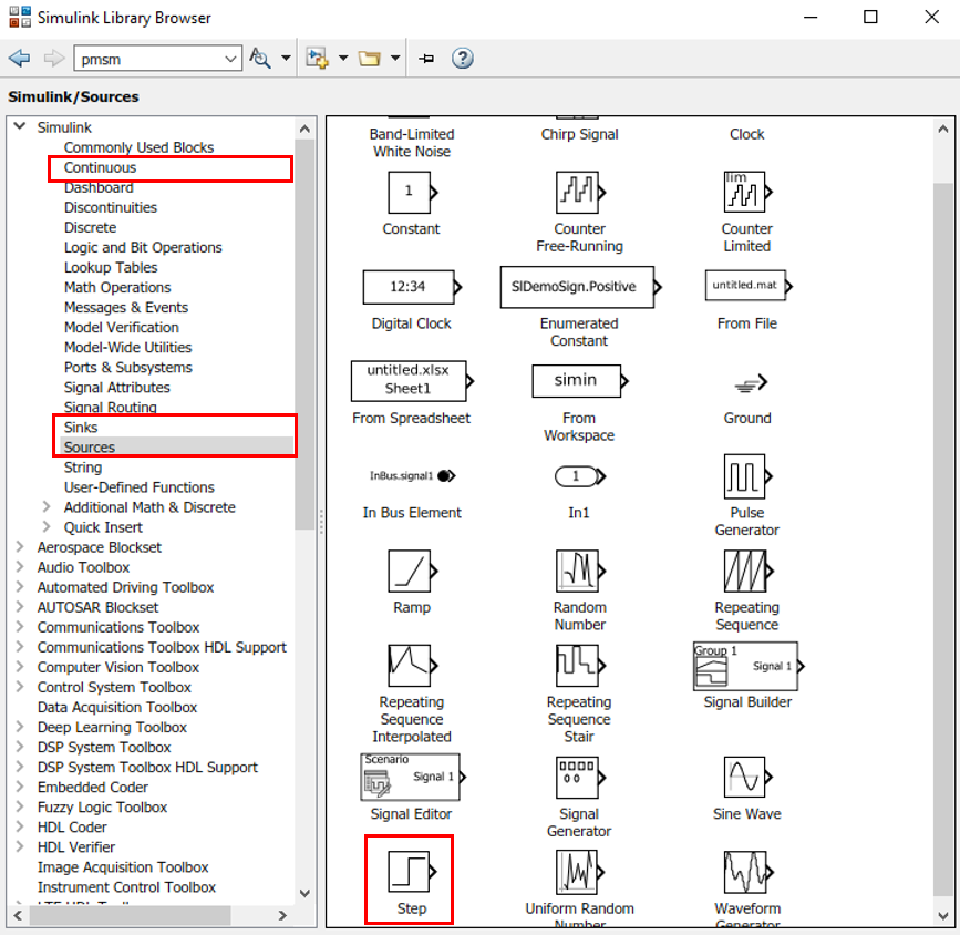
Figure 3. Selecting the required components to implement the system model and applying inputs to it.
After selecting the required components, we connect them to each other as shown in Figure 4. Then, by double-clicking on the TransferFcn block, we enter the parameters of the system’s linearized model into it.
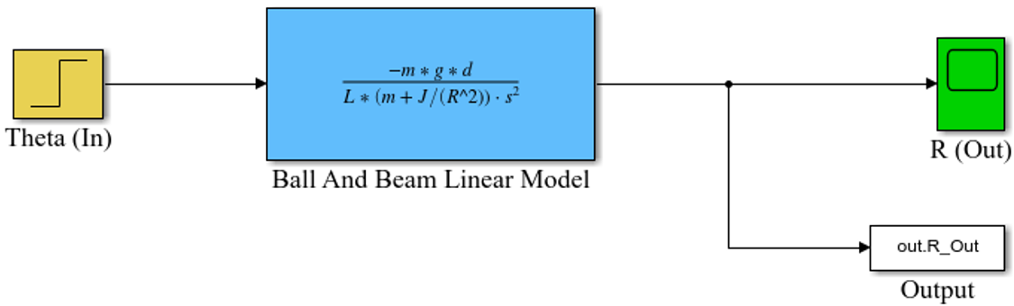
Figure 4. Implementing the open-loop system in the SIMULINK environment.
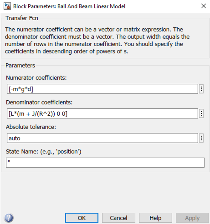
Figure 5. Setting the parameters of the ball and beam system model.
To plot the step response of this system, we use the Step block. The parameters of this block are set according to the configuration shown in Figure 6:
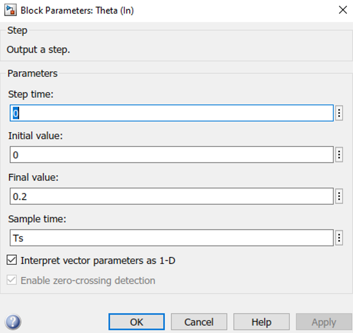
Figure 6. Setting the reference input parameters.
As observed, in the open-loop system simulation, we have considered the reference input as an angular position of 0.2 radians. Additionally, to plot the step response of the system and record the data, we have used the Scope and To Workspace blocks. Using the To Workspace block, the output samples along with the simulation time can be imported into MATLAB’s workspace, allowing the output plot to be generated with higher quality. The settings for this block are shown in Figure 7.
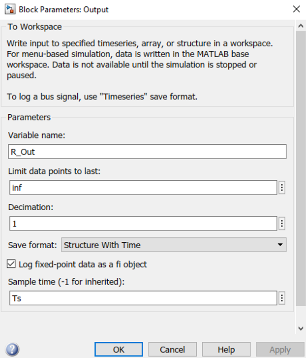
Figure 7. Setting the parameters of the To Workspace block.
To run the simulation, after setting the simulation time in the Stop Time field, we start the simulation by selecting the Run option. Additionally, to plot the output, we execute the following commands in the MATLAB Editor environment:
Time = out.R_Out.time;
R = out.R_Out.signals.values;

figure
plot(Time, R, 'r', 'linewidth', 2)
grid on
xlabel('Time(sec)')
ylabel('R')
title('Output Chart')
legend('R')
The open-loop system output plot for a step input with an amplitude of 0.2 is shown in Figure 8:
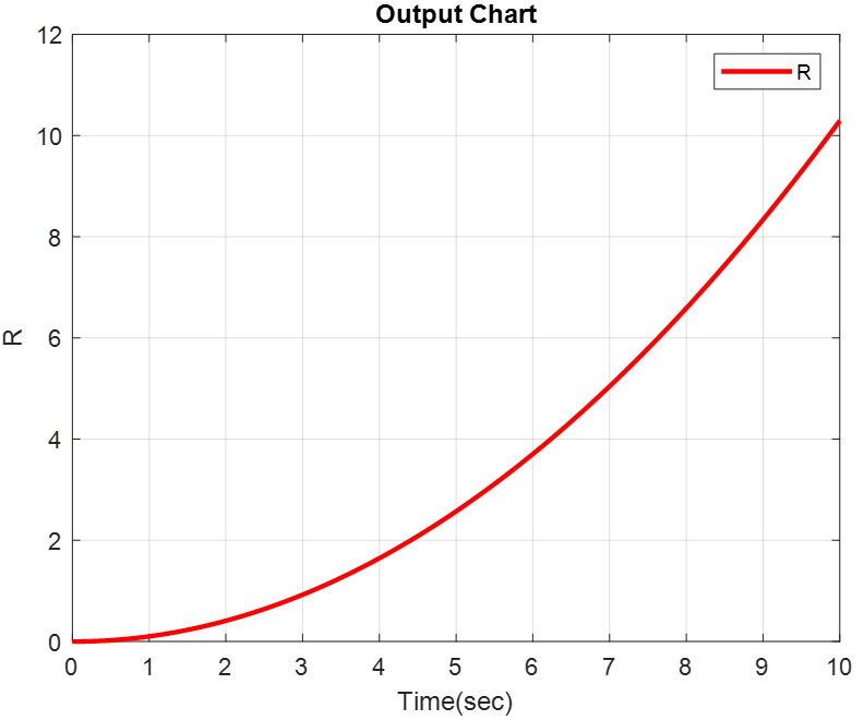
Figure 8. Step response plot of the open-loop system for a step input with an amplitude of 0.2 radians.
Since the open-loop system model includes two pure integrators, as expected, the open-loop system output for a step input has a parabolic shape.
Next, we intend to simulate the closed-loop system. For this purpose, it is necessary to add a summing block (Sum) to the simulation. The closed-loop system along with the proportional controller is shown:
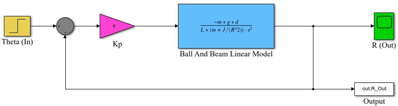
Figure 9. Implementing the closed-loop system with a proportional controller in the SIMULINK environment.
On the other hand, we know that when the open-loop system has two pure integrators, it cannot be controlled using only a single gain, because in this case the closed-loop poles lie on the imaginary axis and the system becomes oscillatory. This can also be analyzed by plotting the root locus. To plot the root locus, we use the rlocus command in MATLAB. The following code is used to plot the root locus of the ball and beam system:
s = tf('s');
G = -m*g*d/(L*(m+J/(R^2))*s^2)

figure(1)
rlocus(G, 'b')
hold on
rlocus(-G, 'r')
legend('k>0', 'k<0')
By running the above program, the root locus plot of this system is generated as shown in Figure 10:
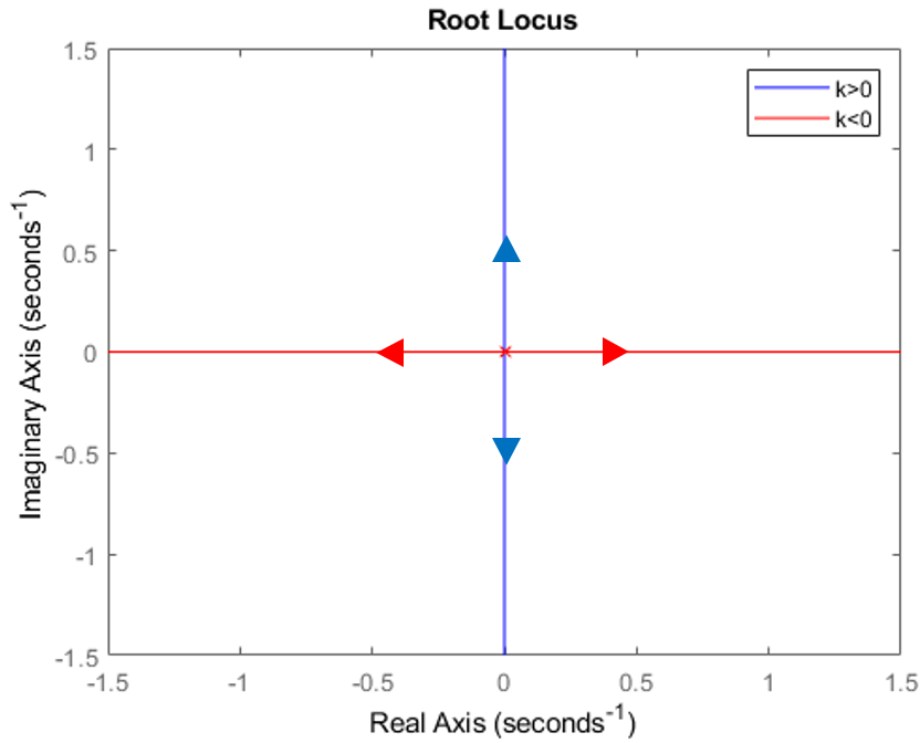
Figure 10. Root locus plot of the ball and beam system.
As observed, for positive gains, the closed-loop poles move along the imaginary axis, causing the system to oscillate. For negative gains, one of the closed-loop poles lies on the right-hand side of the imaginary axis, making the system unstable. Therefore, it is clear that this system cannot be controlled using only a single gain.
Figure 11 shows the closed-loop system response for a proportional controller with a gain of $K_P = 6$.
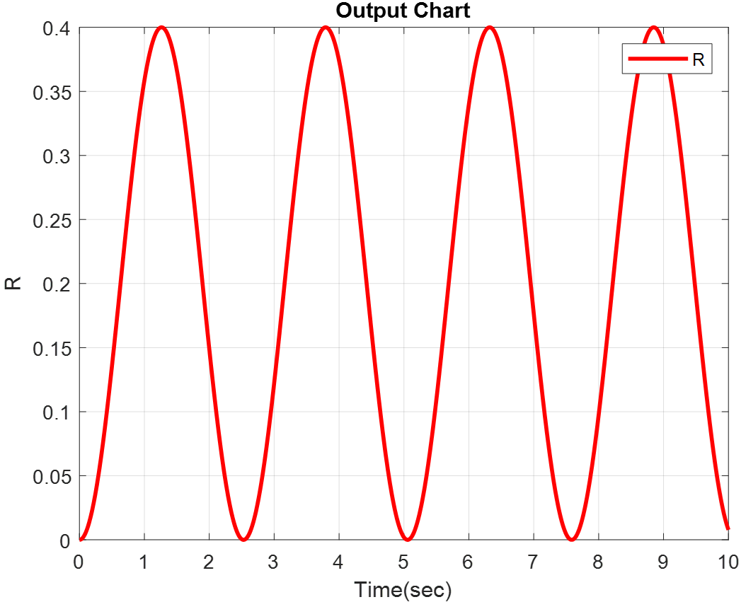
Figure 11. Step response plot of the closed-loop system for a proportional compensator with gain $K_P = 6$.
As observed, the closed-loop system response, as expected, is oscillatory, whereas the control objective was for the output to reach 0.2. Therefore, to achieve this control objective, it is necessary to use a PD or PID controller. Next, we intend to implement the closed-loop system with these two controllers. For designing the controller, MATLAB toolboxes such as PID Tuner or sisotool can be used. For our work, we use PID Tuner. To do this, first open the PID Tuner from the APPs section, and then define the system model using the following commands and import it into the PID Tuner toolbox.
g = -9.8; %Gravitional acceleration (m/s^2).
R = 0.02; %Radius of ball (m).
L = 0.34; %Length of beam (m).
m = 0.0026; %mass of the ball (kg).
d = 0.05; %Lever arm offset (m).
J = 2*m*R^2/5; %Moment of inertia of ball (Kg.m^2).

s = tf('s');
G = -m*g*d/(L*(m+J/(R^2))*s^2)
After setting the parameters, the PD controller gains are obtained as $K_P=7$ and $K_D=5.5$.
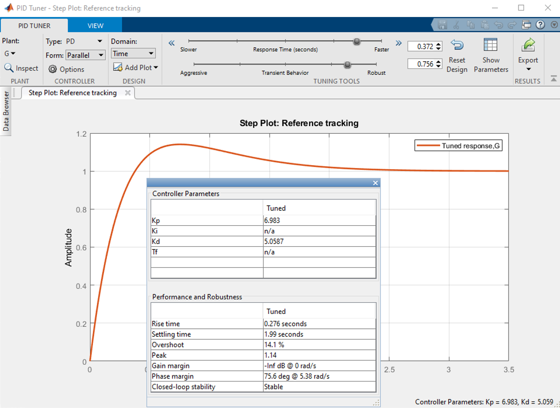
Figure 12. Tuning the control gains using PID Tuner.
After designing the proportional-derivative (PD) controller, we proceed to implement it in the SIMULINK environment. Since a pure differentiator cannot be used in a PD controller (due to its non-causal nature), a fast pole must also be added. Figure 13 shows the block diagram of the closed-loop system with the implemented PD controller.
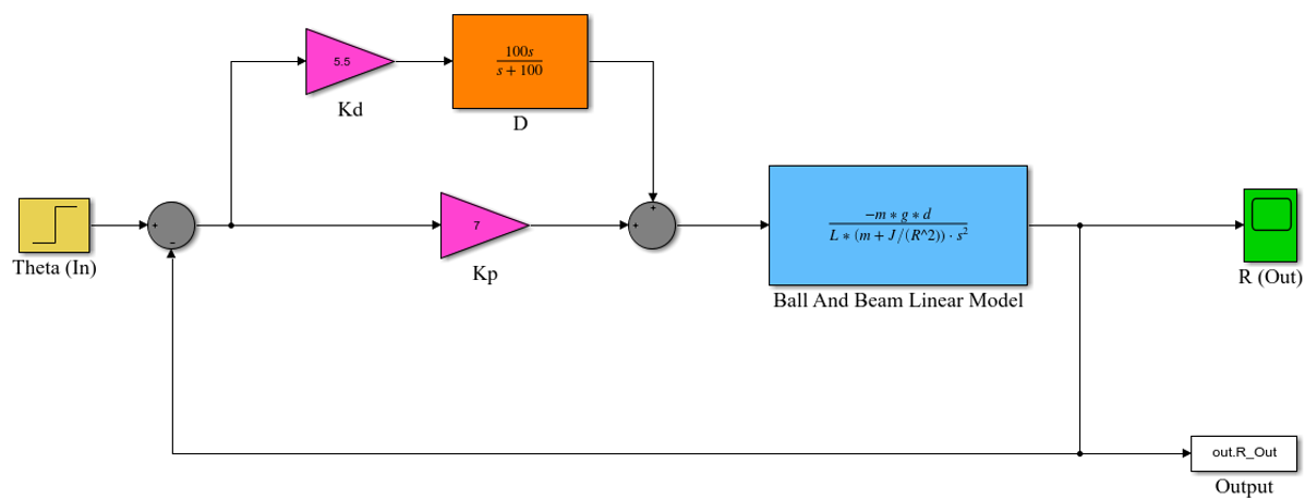
Figure 13. Implementing the closed-loop system with a PD controller in the SIMULINK environment.
By running the simulation of the closed-loop system with the designed PD controller, the step response of the system for a reference input of 0.2 is obtained as shown in Figure 14.
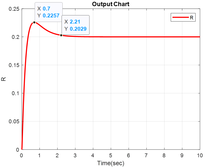
Figure 14. Step response plot of the closed-loop system for a PD controller with gains $K_P=7$ and $K_D=5.5$.
Based on the plot in Figure 14, the response has an overshoot of approximately 14.6% and a settling time of about 2.2 seconds.
Next, using PID Tuner, we design a PID controller. Accordingly, the suitable control gains are obtained as $K_P=15.1$, $K_D=8.4,$ and $K_I=2.9$. We then implement the closed-loop system with the PID controller as shown. Figure 15 presents the block diagram of the closed-loop system with the PID controller.
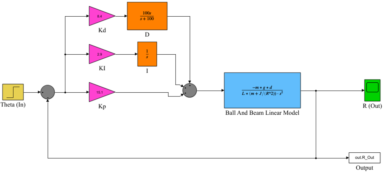
Figure 15. Implementing the closed-loop system with a PID controller in the SIMULINK environment.
By running the simulation of the closed-loop system with the designed PID controller, the step response of the system for a reference input of 0.2 is obtained as shown in Figure 16.
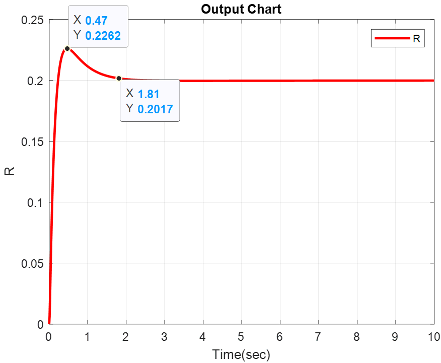
Figure 16. Step response plot of the closed-loop system for a PID controller with gains $K_P=15.1$, $K_D=8.4$ and $K_I=2.9$.
Based on the plot in Figure 16, the response exhibits an overshoot of approximately 13.1% and a settling time of about 1.81 seconds. As observed, when using the PID controller, the system’s overshoot is reduced and the response speed increases; however, adding the integral component raises the overall cost of the controller. Therefore, to achieve the desired response, the PD controller alone is sufficient.